Understanding Forward-Forward Algorithm
Paper author: Geoffrey Hinton
Publish date: 2022-12-27
Link to the paper: Forward-Forward Paper
TL;DR
-
The new Forward-Forward optimization algorithm is a novel learning procedure for neural networks that replaces the forward and backward passes of back-propagation with two forward passes, one performed with positive (real) data and the other one performed with negative (synthesized/wrongly labelled) data
-
Instead of computing a cumulative loss function, whose gradient is back-propagated through all the layers, with Forward-Forward each layer has its own objective, i.e. norm of positive samples vector
-
Forward-Forward reduces the memory consumption of back-propagation, while obtaining comparable performance to its counterpart. However back-propagation is still preferrable when resources are not limited
-
Being an introductory exploration, the Forward-Forward has not been tested in enough different scenarios yet to be considered a reliable solution for training a neural network
In this article we’re going to talk about the newly developed Forward-Forward algorithm, which should serve as an alternative to the back-propagation learning algorithm. Specifically, in this post I focus on the motivations behind its use-cases and I provide an explanation on how the algorithm works, compared to back-propagation one.
Motivations
Before delving into the pros of the Forward-Forward Algorithm, it is useful to grasp some of the common flaws of back-propagation, which limitates its use in certain situations.
Drawbacks of back-propagation
Despite being the most popular algorithm used to train neural networks, back-propagation presents some critical flaws which have not been addressed yet. Let’s explore them.
Initially, neural networks were developed with the hope of mimicking human brain behavior, as the concepts of neurons and layers are highly correlated with our understanding of actual neurons and cortical layers. Based on these assumptions, we would prefer to have a training algorithm that closely resembles the training process in the human brain itself.
However, there is "no convincing evidence that cortex explicitly propagates error derivatives or stores neural activities for use in a subsequent backward pass". The top-down connections in the visual system do not follow the expected pattern of bottom-up connections, making back-propagation unlikely. Instead, they form loops, with neural activity passing through several cortical layers in both areas before returning.
This challenges the feasibility of back-propagation for learning sequences. To process a continuous stream of sensory input without interruptions, the brain needs to streamline data flow and employ a real-time learning mechanism, rather than relying on back-propagation.
Another significant drawback of back-propagation is its dependence on having complete knowledge of the calculations made during the forward pass to calculate accurate derivatives. If we introduce a black box into the forward pass, back-propagation becomes unfeasible unless we can develop a differentiable model for that black box. Interestingly, for the Forward-Forward Algorithm, the presence of a black box doesn’t alter the learning process whatsoever, as there’s no need for back-propagation through it.
One last fundamental drawback is the memory usage. Back-propagation requires storing activations of all intermediate layers. This practical concern becomes evident when aiming to implement deep neural architectures in a production environment where efficiency is a requisite. In such scenarios, the challenges associated with deploying and maintaining these deep models become even more pronounced, potentially affecting the efficiency and agility of the production pipeline.
An interesting property of Forward-Forward
The primary concept behind Forward-Forward is to eliminate the necessity for a complete computational graph of the model when performing a training step. This enables independent training of intermediate layers in any neural network while avoiding the storage of all intermediate computations.
This approach results in a more streamlined training algorithm, which can prove highly effective in situations where certain parts of the model are non-differentiable or when the training environment has limited performance.
How it works?
Now, before discussing how Forward-Forward algorithm works, let’s explore the inner processes of back-propagation, which is fundamental to understand the improvements that Forward-Forward proposes.
Inside back-propagation
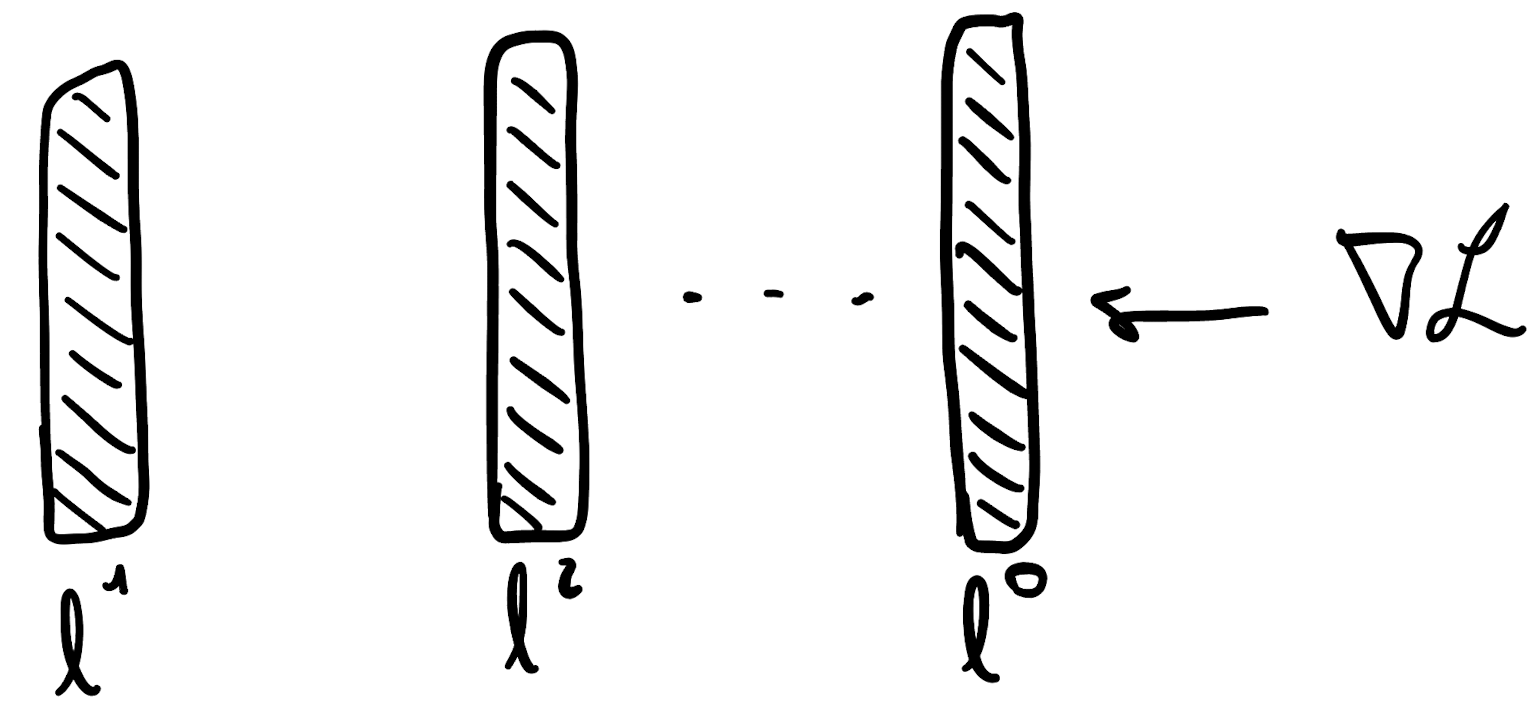
A back-propagation algorithm involves three main steps, depicted below.
- In the first step the input is propagated through the model computing all the intermediate activations (and storing them) and the output.

- In the second step, depending on the task (classification or regression) a loss function (Cross Entropy in the example) is used to compute the loss/distance between the outputs and the desired results. The aggregated loss (sum of distances) is then used to perform a learning step of the model.
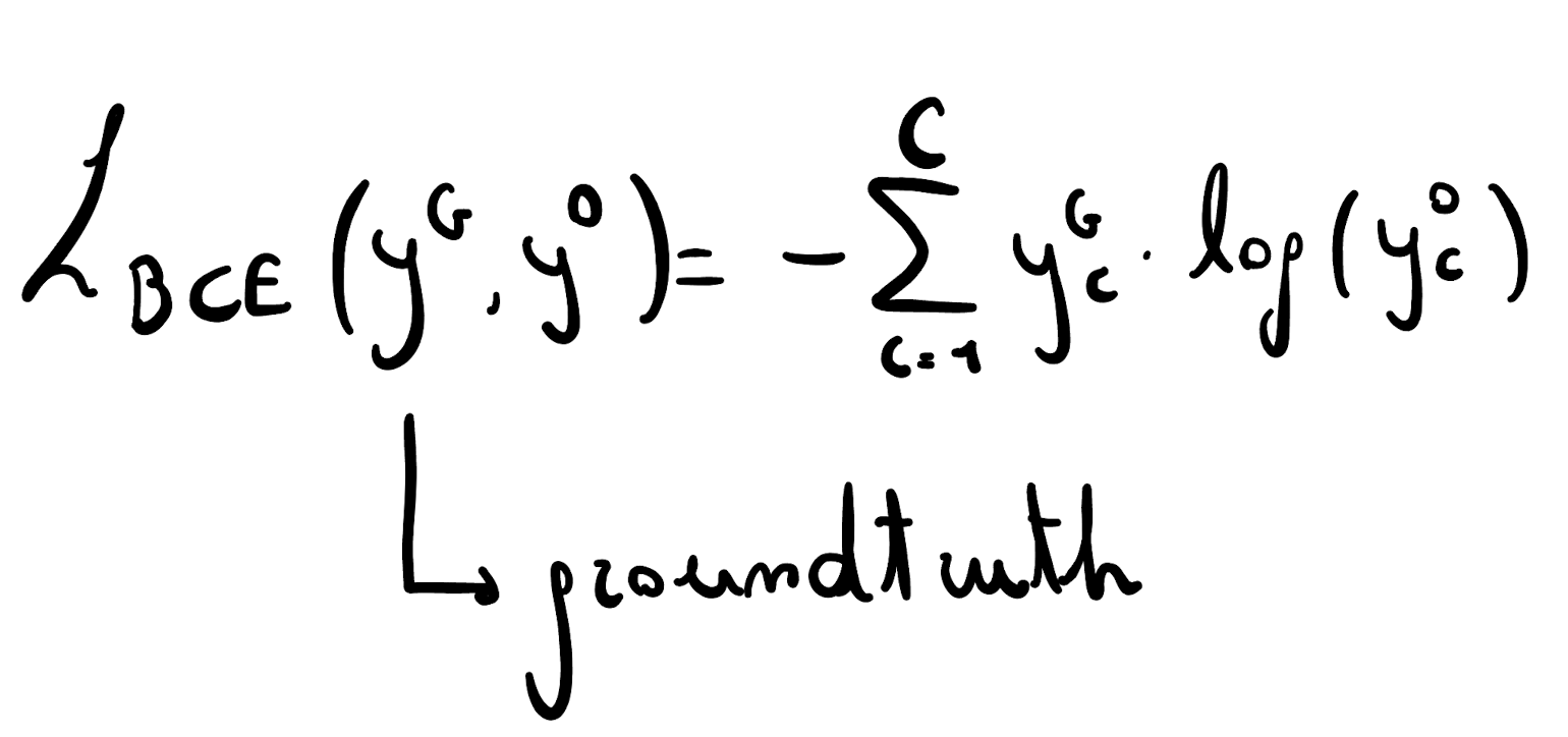
- In the third step the gradient of the loss is computed (direction of max increase) and is propagated to all the parameters of the model. Here the idea is to find the contribution of each weight in the final value of the loss, by decomposing the entire loss gradient using the chain rule. Once each contribution (given the input) is computed, all the weights are updated by \(- \lambda \cdot \partial L_{CE}\), where \(\lambda\) is a scalar that represents the learning rate.
The Forward-Forward
The Forward-Forward algorithm draws inspiration from Boltzmann machines (Hinton and Sejnowski, 1986) and Noise Contrastive Estimation (Gutmann and Hyvärinen, 2010). This approach replaces the traditional forward and backward passes in backpropagation with two forward passes. These two passes are identical in operation but differ in their data source and objectives.
The positive pass processes actual data, adjusting weights to enhance the goodness in each hidden layer. Conversely, the negative pass deals with “negative data” and tunes weights to diminish the quality in each hidden layer.
Let’s now take a look on the inner working of a forward pass by analyzing what happens inside a single layer. Given the layer independence property of Forward-Forward, understanding the inner working of one layer is equal to understand how the entire process works.
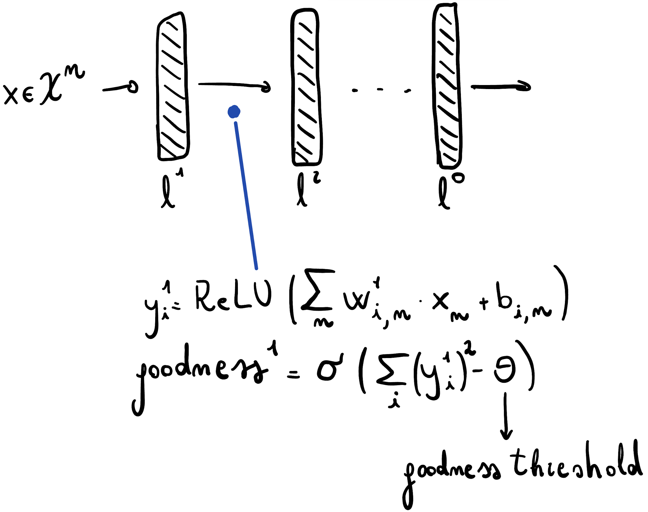
Initially, a positive input is provided to the network and an intermediate representation \(y_i^1\) is obtained. The goodness score of the input at the given layer (\(goodness^1\)) is then computed as the sigmoid of the norm of the input vector minus a decision threshold (which is an hyperparameter). Defining the goodness as the norm of the vector (or length of the vector, for those who prefer such phrasing) is not mandatory, but appears to be quite useful.
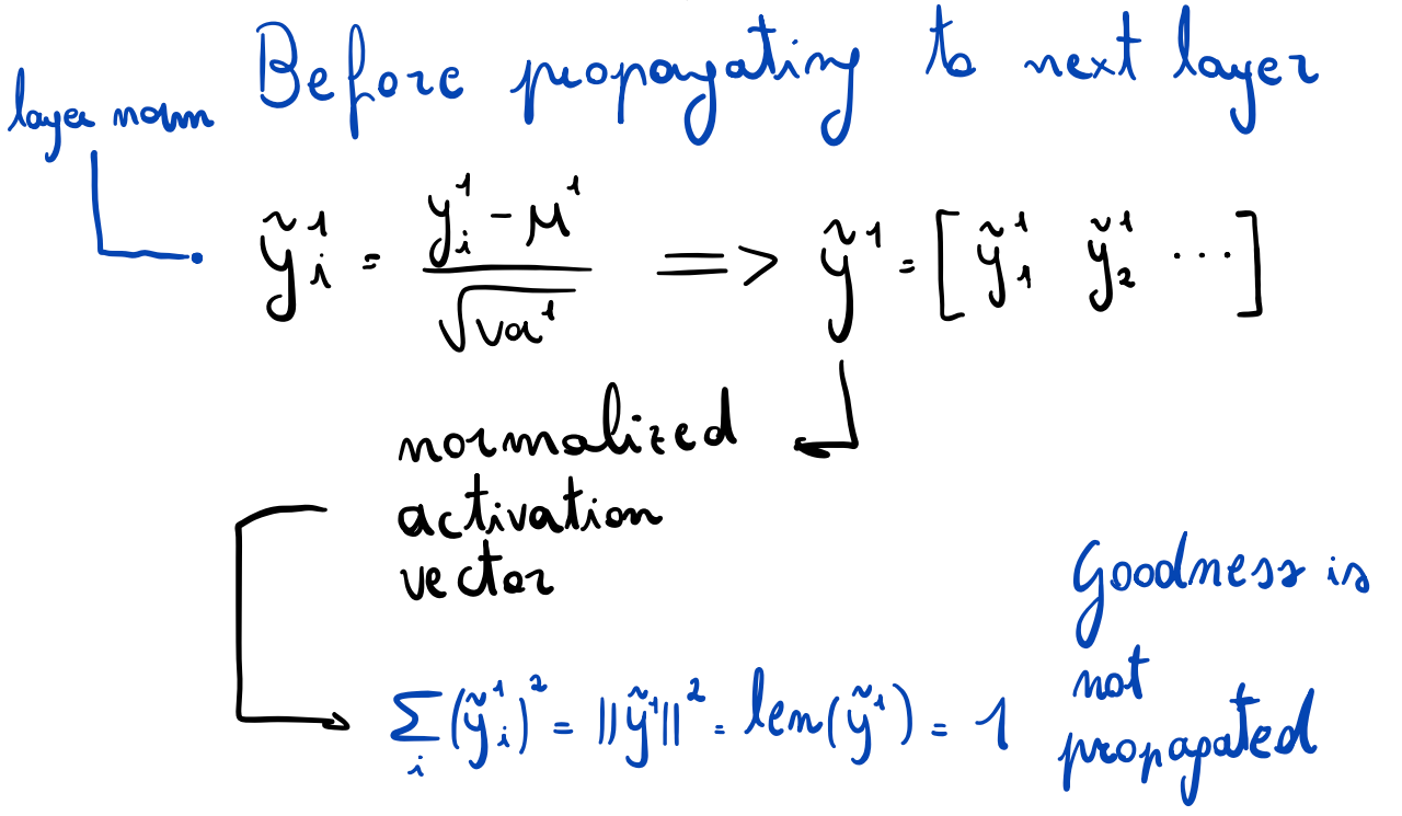
As I mentioned before, one of our goal is to obtain layers independence at training/inference time, which guarantess that less resources are employed to run a model. Now, if after the first layer we would simply propagate the vector through the next layers, what would avoid the network to learn the identity vector? If we think about it, it would be computationally cheaper, once reached a positive goodness at a layer \(L\), to keep all the \(l > L\) layers’ weights equal to \(\mathbb{1}\). In order to circumvent this behaviour and propagate only a useful part of the original input, a layer normalization step is applied. The formula, which is depicted in the figure below, returns the normalized input vector. The goodness (i.e. the length) is then “removed” before the propagation, but the original information (given by the direction of the vector) is preserved for the next steps.
Let’s now take a look to what a positive sample (in supervised learning) is. In the original paper, Hinton proposes to use the first \(C\) of the image to encode in a one-hot fashion the class corresponding to the object in the picture. Conversely, negative data can be either a perturbated image with the correct label or the same image with a wrong label. The ultimate goal is to have a degree of wrongness that can be used by the model to learn that wrong/negative data should have lower goodness (or higher wrongness). As in the unsupervised paradigm no labels are provided, the concept of wrongness can be crafted either by adding noise or by interpolating two positive images.
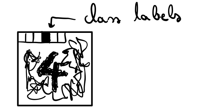
In this current formulation, Forward-Forward applied to feed-forward networks avoid to later layers to affect what is learned in earlier layers. Despite this being the key for the layer independence, this prevent the model to learn patterns as a whole. To solve this, Hinton proposes to employ a multi-layer recurrent neural network (rnn) architecture where the input is a boring video made up of a repeat image.
RNN allows connectivity at different time-step by design and this consent to learn patterns as a whole, without replacing the layer independency of Forward-Forward. Applied to rnn architecture, the Forward-Forward become Forward-Forward in time.
Future works
As this is a preliminary exploration, Hinton concludes the paper by presenting a set of intriguing questions that are slated for future investigation. I present them in their original wording because I think they can be an engaging prompt for anyone who reads my article.
-
Can FF produce a generative model of images or video that is good enough to create the negative data needed for unsupervised learning?
-
What is the best goodness function to use? This paper uses the sum of the squared activities in most of the experiments but minimizing the sum squared activities for positive data and maximizing it for negative data seems to work slightly better. More recently, just minimizing the sum of the unsquared activities on positive data (and maximizing on negative) has worked well
-
What is the best activation function to use? So far, only ReLUs have been explored. There are many other possibilities whose behaviour is unexplored in the context of FF. Making the activation be the negative log of the density under a t-distribution is an interesting possibility (Osindero et al., 2006).
-
For spatial data, can FF benefit from having lots of local goodness functions for different regions of the image (Löwe et al., 2019)? If this can be made to work, it should allow learning to be much faster.
-
For sequential data, is it possible to use fast weights to mimic a simplified transformer (Ba et al., 2016a)?
-
Can FF benefit from having a set of feature detectors that try to maximize their squared activity and a set of constraint violation detectors that try to minimize their squared activity (Welling et al., 2003)?
Conclusions
In this post I brought the attention to an interesting algorithm for training neural networks, called Forward-Forward. Conceptually this novel paradigm is orthogonal to the back-propagation one, allowing for independent layer learning and improved memory efficiency. Despite being a good alternative in some specific contexts (low-power/low-sepcs), when back-propagation requirements are matched it still outperforms the novel Forward-Forward, suggesting that many iterations are still required to make it useful in real-life scenarios.
Despite back-propagation seems to dominate in the realm of learning algorithms, the process of research works by little and apparently meaningless steps, which over time leads to greater discoveries and disruptive paradigm shifts.
To this extent, Forward-Forward perfectly represents a curious perspective in machine learning that is just waiting to be harnessed and improved, like every new discovery.